Unlock Probability: Calculate with Mean & SD Like a Pro!

Statistical analysis relies on understanding probability distributions. Mean and Standard Deviation (SD), vital parameters within these distributions, influence probability calculations. In data science, professionals commonly leverage these measures. How to calculate probability with mean and sd is a core competence. This article will explore this concept, making it simple to apply to your analyses. The Z-table will be explained as a tool to look up the corresponding probability value once the Z-score is found.

In an increasingly data-driven world, the ability to understand and interpret probabilities has become an indispensable skill across numerous fields. From finance to healthcare, engineering to marketing, probability calculations underpin critical decision-making processes, enabling professionals to navigate uncertainty and make informed choices. This exploration delves into the essential role of mean and standard deviation in unlocking the true potential of probability, transforming raw data into actionable insights.

The Ubiquity of Probability

Probability is not confined to the realm of theoretical mathematics; it is a fundamental aspect of our daily lives and professional endeavors. Understanding probability allows us to:

• Assess Risk: In finance, it’s crucial for evaluating investment risks, pricing options, and managing portfolios.

• Improve Outcomes: In healthcare, it helps in assessing the effectiveness of treatments, predicting disease outbreaks, and personalizing patient care.

• Optimize Processes: In engineering and manufacturing, it aids in quality control, reliability analysis, and process optimization.

• Target Audiences: In marketing, it is essential for predicting consumer behavior, optimizing advertising campaigns, and personalizing customer experiences.

Without a grasp of probability, we are left to rely on intuition and guesswork, which can lead to suboptimal outcomes and missed opportunities.

Mean and Standard Deviation: The Cornerstones of Insight

While probability provides a framework for understanding uncertainty, mean and standard deviation serve as essential tools for quantifying and interpreting data within that framework.

• The Mean: Often referred to as the average, provides a measure of central tendency, indicating the typical value within a dataset.

• The Standard Deviation: Quantifies the spread or variability of data around the mean, revealing how tightly or loosely data points are clustered.

Together, these measures provide a powerful lens through which to examine probability distributions, allowing us to understand not only the likelihood of events but also the range of possible outcomes and their associated variability.

From Data to Decisions: Extracting Meaningful Insights

The true power of mean and standard deviation lies in their ability to transform raw data into meaningful insights that drive informed decisions. By understanding the central tendency and variability of data, we can:

• Identify Trends: Spot patterns and anomalies that would otherwise go unnoticed.

• Make Predictions: Forecast future outcomes based on historical data.

• Evaluate Performance: Compare different scenarios and assess their relative effectiveness.

• Optimize Strategies: Refine approaches based on data-driven evidence.

By leveraging these measures, we can move beyond simply collecting data to actively using it to improve our understanding of the world and make better decisions in the face of uncertainty. The subsequent sections will delve deeper into the practical applications of mean and standard deviation in probability calculations, equipping you with the knowledge and skills to unlock the full potential of your data.

While probability provides a framework for understanding uncertainty, mean and standard deviation serve as essential tools for quantifying and interpreting data within that framework. Now, let’s clearly define the fundamental building blocks: probability itself, the mean, and the standard deviation. These concepts are not just theoretical constructs; they are the keys to unlocking actionable insights from data.

Fundamentals Demystified: Probability, Mean, and Standard Deviation Explained

At the heart of understanding probability lies a set of core concepts. These concepts, while seemingly simple, are crucial for anyone looking to make sense of the world through data. Probability, mean, and standard deviation are the cornerstones upon which many statistical analyses are built. Understanding each, and how they relate, will empower you to move beyond simply collecting data, towards truly interpreting it.

Defining Probability: A Concise Review

Probability, at its most basic, is a measure of the likelihood of an event occurring. It’s expressed as a number between 0 and 1, where 0 indicates impossibility and 1 indicates certainty.

A probability of 0.5 suggests an equal chance of the event happening or not happening.

Understanding probability requires grasping related concepts like:

• Sample Space: The set of all possible outcomes of an experiment.
• Event: A subset of the sample space, representing a specific outcome or group of outcomes.
• Independent Events: Events whose outcomes do not affect each other.

These building blocks are essential for calculating and interpreting probabilities accurately.

Defining Mean: The Average Value

The mean, often referred to as the average, is a measure of central tendency. It represents the typical value within a dataset.

Calculated by summing all the values and dividing by the number of values, the mean provides a single number that summarizes the center of a distribution.

While it’s a useful measure, it’s important to remember that the mean can be influenced by extreme values (outliers). Therefore, it’s often used in conjunction with other measures to gain a more complete understanding of the data.

Defining Standard Deviation: Measuring Data Spread

Standard deviation quantifies the spread or variability of data points around the mean.

A low standard deviation indicates that data points are clustered closely around the mean, suggesting a more consistent dataset. Conversely, a high standard deviation suggests that data points are more dispersed, indicating greater variability.

The standard deviation is crucial for understanding the distribution of data and for assessing the reliability of the mean as a representative value.

It is calculated as the square root of the variance, which is the average of the squared differences from the mean. This ensures that both positive and negative deviations contribute to the overall measure of spread.

Mean and Standard Deviation: Providing Context to Probability

Probability calculations become significantly more meaningful when considered in the context of the mean and standard deviation.

• Mean as a Reference Point: The mean serves as a benchmark, allowing us to assess how likely it is for a data point to fall above or below a certain value.

• Standard Deviation as a Scale: The standard deviation provides a scale for measuring how far away a data point is from the mean, allowing us to determine its relative likelihood.

For instance, if we know the mean and standard deviation of a dataset, we can use probability to determine the likelihood of observing a value that is several standard deviations away from the mean. This ability to quantify the unusualness of an event is a powerful tool in many fields, from quality control to risk management.

Defining the mean and standard deviation sets the stage for a deeper exploration into how data is distributed. These measures are particularly powerful when applied to a specific type of distribution – one that appears frequently in nature and statistics.

The Normal Distribution: Your Gateway to Probability Calculations

The Normal Distribution, often called the bell curve, is a cornerstone of statistical analysis and, consequently, probability calculations. Its ubiquitous presence in various fields stems from its ability to model many real-world phenomena. Understanding the Normal Distribution is paramount to unlocking advanced probability calculations and gaining deeper insights from data.

Importance of the Bell Curve

The Normal Distribution is important because it simplifies complex data sets into a manageable and predictable form. It’s a symmetrical distribution where most values cluster around the mean.

This inherent structure enables us to:

• Estimate probabilities accurately.
• Make informed decisions based on sample data.
• Draw inferences about populations.

Its widespread applicability makes it an indispensable tool for researchers, analysts, and decision-makers across disciplines.

Key Characteristics of the Normal Distribution

The Normal Distribution possesses unique characteristics that define its shape and behavior. These characteristics include symmetry, the relationship between the mean, median, and mode, and the defining role of standard deviation.

Symmetry

The Normal Distribution is perfectly symmetrical around its mean. This symmetry means that the left and right halves of the curve are mirror images of each other. This also signifies that values are equally likely to occur above or below the mean.

Mean, Median, and Mode

In a Normal Distribution, the mean, median, and mode are all equal. This convergence at a single point further emphasizes the distribution’s symmetry and balance. This property simplifies calculations and interpretations, making the Normal Distribution an ideal model for various datasets.

Standard Deviation and Shape

The standard deviation dictates the spread or width of the Normal Distribution. A smaller standard deviation results in a narrower, taller curve, indicating that data points are closely clustered around the mean.

Conversely, a larger standard deviation produces a wider, flatter curve, suggesting greater variability in the data. The standard deviation is critical for understanding how data deviates from the average value.

Visualizing Data: Mean and Standard Deviation

Visualizing the Normal Distribution helps solidify the understanding of how mean and standard deviation affect its appearance and interpretability. The mean positions the curve along the x-axis, while the standard deviation controls its dispersion.

For example, consider two Normal Distributions with the same mean but different standard deviations. The distribution with the smaller standard deviation will appear more concentrated around the mean, while the distribution with the larger standard deviation will be more spread out.

Similarly, if two Normal Distributions have the same standard deviation but different means, they will have the same shape but will be centered at different points along the x-axis. By understanding these visual relationships, you can quickly assess and interpret data distributions.

Defining the mean and standard deviation sets the stage for a deeper exploration into how data is distributed. These measures are particularly powerful when applied to a specific type of distribution – one that appears frequently in nature and statistics.

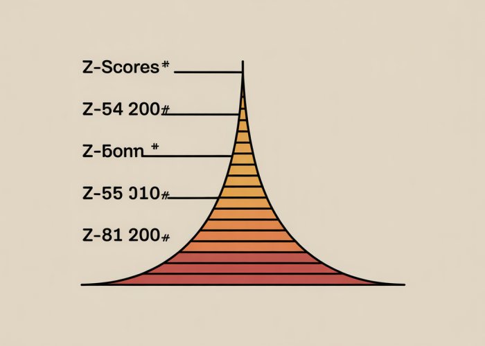
Calculating Probabilities with Z-Scores: A Step-by-Step Guide

The Normal Distribution, as we’ve seen, provides a framework for understanding data. However, to pinpoint the likelihood of a specific value or range of values occurring, we need a more precise tool. That’s where Z-scores enter the picture, offering a standardized method for calculating probabilities associated with any normal distribution.

What is a Z-score?

A Z-score, also known as a standard score, quantifies the number of standard deviations a particular data point deviates from the mean of its distribution. In simpler terms, it tells us how "unusual" a specific value is.

A Z-score of 0 indicates that the data point is exactly at the mean.

A positive Z-score means the data point is above the mean.

Conversely, a negative Z-score indicates that it’s below the mean.

The purpose of the Z-score is to standardize any normal distribution, regardless of its original mean and standard deviation, into a standard normal distribution with a mean of 0 and a standard deviation of 1. This standardization allows us to use a single, universal table (the Z-table) to find probabilities.

The Z-score Formula: A Step-by-Step Guide to Calculation

The Z-score formula is straightforward:

Z = (X – μ) / σ

Where:

• Z is the Z-score.
• X is the individual data point.
• μ (mu) is the population mean.
• σ (sigma) is the population standard deviation.

Let’s break down how to apply this formula:

1. Identify the Data Point (X): Determine the specific value you want to analyze.
2. Determine the Mean (μ): Find the average value of the dataset.
3. Find the Standard Deviation (σ): Calculate the standard deviation, which measures the data’s spread.
4. Apply the Formula: Subtract the mean from the data point (X – μ), then divide the result by the standard deviation (σ).

The resulting Z-score represents how many standard deviations away from the mean your data point is.

Using Z-scores to Find Probabilities: Using Z-scores and Normal Distribution tables

Once you have your Z-score, you can use a standard normal distribution table (also known as a Z-table) to find the probability associated with that score. A Z-table provides the area under the standard normal curve to the left of a given Z-score, which represents the cumulative probability.

Here’s how to use the Z-table:

1. Locate the Z-score: Find the Z-score in the table. Z-tables typically have Z-scores listed in the first column and first row.
2. Read the Probability: The corresponding value at the intersection of the row and column represents the probability of observing a value less than or equal to your chosen data point.

Note: Z-tables usually give the area to the left of the Z-score.

To find the area to the right, subtract the value from the table from 1.

Example: Calculate the Probability of a Value within a Range

Let’s say we have a dataset of test scores with a mean (μ) of 75 and a standard deviation (σ) of 10. We want to find the probability of a student scoring 80 or less.

1. Calculate the Z-score:

   Z = (80 – 75) / 10 = 0.5

2. Use the Z-table: Look up the Z-score of 0.5 in the Z-table.

   The corresponding probability is approximately 0.6915.

3. Interpret the Result: This means there’s approximately a 69.15% chance that a student will score 80 or less.

Now, let’s calculate the probability of a student scoring above 80. Since the Z-table gives the area to the left, we subtract our previous result from 1.

1 – 0.6915 = 0.3085

Therefore, there is a 30.85% chance that a student will score above 80.

Understanding and applying Z-scores, along with mastering the use of the Normal Distribution table, provides a powerful method for probability calculation that transforms raw data into actionable insights.

The Empirical Rule: Quick Probability Estimations

While Z-scores offer a precise method for pinpointing probabilities within a normal distribution, there exists a handy shortcut for quicker estimations: the Empirical Rule. This rule, also known as the 68-95-99.7 rule, provides a simple yet powerful way to understand data spread and estimate probabilities without complex calculations.

Understanding the Empirical Rule

The Empirical Rule applies specifically to normal distributions and describes the percentage of data that falls within certain standard deviations from the mean.

• Approximately 68% of the data falls within one standard deviation of the mean (μ ± 1σ).

• Approximately 95% of the data falls within two standard deviations of the mean (μ ± 2σ).

• Approximately 99.7% of the data falls within three standard deviations of the mean (μ ± 3σ).

This rule provides a quick visual and mental model of how data is distributed around the average.

Applications of the Empirical Rule

The Empirical Rule’s simplicity makes it incredibly useful for rapid assessments and estimations in various scenarios.

For example, imagine a dataset of student test scores with a mean of 75 and a standard deviation of 5.

Using the Empirical Rule, we can quickly estimate that approximately 68% of students scored between 70 and 80.

Similarly, about 95% scored between 65 and 85.

This allows for quick, high-level insights without needing to calculate individual Z-scores.

It is important to remember that the Empirical Rule provides estimations, not exact probabilities.

Calculating Probabilities with the Empirical Rule

Applying the Empirical Rule to calculate probabilities involves understanding the symmetrical nature of the normal distribution.

Since the rule tells us the percentage of data within a certain range of standard deviations from the mean, we can also deduce the percentage of data outside that range.

For instance, if 68% of data falls within one standard deviation, then 32% falls outside of it.

This 32% is split equally between the two tails of the distribution, meaning 16% lies below μ – 1σ and 16% lies above μ + 1σ.

Similarly, if 95% of the data lies within two standard deviations, then 5% lies outside.

Dividing this gives 2.5% in each tail.

Z-Scores vs. Empirical Rule: Choosing the Right Tool

The Empirical Rule provides a rapid, intuitive way to estimate probabilities.

However, it only offers approximations for values that fall exactly one, two, or three standard deviations from the mean.

For probabilities associated with values falling between these standard deviations, or for a more precise calculation, Z-scores and the Z-table become necessary.

• Use the Empirical Rule for quick estimations and a general understanding of data spread around the mean.

• Use Z-scores for precise probability calculations and when dealing with values that don’t fall neatly at one, two, or three standard deviations from the mean.

In essence, the Empirical Rule serves as a valuable mental shortcut, while Z-scores provide the accuracy required for more in-depth analysis. Choosing the right tool depends on the desired level of precision and the context of the situation.

Central Limit Theorem: Expanding Your Probability Toolkit

Having explored the Empirical Rule as a method of approximation, we can now delve deeper into a more powerful and versatile tool: the Central Limit Theorem (CLT). This theorem acts as a cornerstone of statistical inference, allowing us to make inferences about population parameters based on sample data, even when the population distribution is unknown.

Understanding the Central Limit Theorem

The Central Limit Theorem (CLT) is a fundamental concept in statistics, with far-reaching implications. It states that the distribution of sample means will approach a normal distribution, regardless of the shape of the population distribution, as the sample size increases. This holds true, provided the samples are random and independent.

Let’s break this down further:

• Population Distribution: This is the distribution of all individual values in the entire population. It could be normal, uniform, exponential, or any other shape.

• Sample: A subset of the population selected for analysis.

• Sample Mean: The average of the values in a single sample.

• Sampling Distribution of the Sample Means: The distribution formed by the means of all possible samples of a given size taken from the population.

The CLT essentially says that even if the population distribution is not normal, the sampling distribution of the sample means will be approximately normal if the sample size is large enough. What constitutes a "large enough" sample size? A common rule of thumb is that a sample size of n ≥ 30 is generally sufficient for the CLT to hold.

How Sample Means Relate to the Population Mean

One of the most powerful aspects of the CLT is its connection between sample means and the population mean.

The theorem states that the mean of the sampling distribution of the sample means is equal to the population mean (μ).

In other words, if you were to take many random samples from a population, calculate the mean of each sample, and then calculate the average of all those sample means, that average would be very close to the true population mean. This holds true irrespective of the population.

Furthermore, the CLT also describes the standard deviation of the sampling distribution of the sample means, which is often referred to as the standard error of the mean. The standard error is calculated as:

σ_x̄ = σ / √n

Where:

• σ_x̄ is the standard error of the mean.
• σ is the population standard deviation.
• n is the sample size.

This formula shows that as the sample size increases, the standard error decreases.

This means that the sample means tend to cluster more closely around the population mean when the sample size is larger, resulting in a more precise estimate of the population mean.

Calculating Probabilities for Sample Means Using the Central Limit Theorem

The Central Limit Theorem allows us to calculate probabilities related to sample means, even when we don’t know the distribution of the underlying population. Here’s how to leverage the theorem for probability calculations:

1. Define the Problem: Clearly state the question you’re trying to answer.

   For example, "What is the probability that the average weight of a sample of 50 apples will be greater than 150 grams, given that the population mean weight is 145 grams and the population standard deviation is 20 grams?"

2. Check Conditions: Ensure that the CLT conditions are met. The samples must be random and independent, and the sample size should generally be greater than or equal to 30.

3. Calculate the Standard Error: Use the formula σ_x̄ = σ / √n to calculate the standard error of the mean.

   In our example, σ_x̄ = 20 / √50 ≈ 2.83 grams.

4. Calculate the Z-score: Calculate the Z-score for the sample mean you are interested in using the following formula:

   Z = (x̄ – μ) / σ_x̄

   Where:

   • x̄ is the sample mean you are interested in.
   • μ is the population mean.
   • σ_x̄ is the standard error of the mean.

   In our example, Z = (150 – 145) / 2.83 ≈ 1.77.

5. Find the Probability: Use a Z-table or a statistical software package to find the probability associated with the calculated Z-score.

   In our example, the probability of a Z-score being greater than 1.77 is approximately 0.0384.

   Therefore, the probability that the average weight of a sample of 50 apples will be greater than 150 grams is approximately 3.84%.

By applying the Central Limit Theorem, we can make probabilistic statements about sample means, even when we lack detailed knowledge about the population distribution. This capability significantly expands our ability to analyze data and draw meaningful conclusions.

Central Limit Theorem: Expanding Your Probability Toolkit
Having explored the Empirical Rule as a method of approximation, we can now delve deeper into a more powerful and versatile tool: the Central Limit Theorem (CLT). This theorem acts as a cornerstone of statistical inference, allowing us to make inferences about population parameters based on sample data, even when the population distribution is unknown.

Probability Density Function: Unveiling Continuous Probabilities

While discrete probability deals with distinct, countable outcomes, many real-world scenarios involve continuous data. This is where the Probability Density Function (PDF) comes into play, allowing us to analyze probabilities associated with continuous variables.

Understanding the Probability Density Function

The PDF, often denoted as f(x), is a function that describes the relative likelihood for a continuous random variable to take on a given value. It’s crucial to remember that the PDF itself doesn’t directly represent probability.

Instead, the area under the curve of the PDF over a specific interval gives the probability that the variable falls within that interval.

The total area under the entire PDF curve must equal 1, reflecting the certainty that the variable will take on some value within its possible range.

Connecting Continuous Data and Probabilities

Unlike discrete probability distributions where we can directly calculate the probability of a specific outcome (e.g., the probability of rolling a 3 on a die), continuous variables can take on an infinite number of values.

Therefore, it doesn’t make sense to talk about the probability of a continuous variable being exactly equal to a particular value.

Instead, we focus on the probability of the variable falling within a defined range. The PDF provides the mathematical framework for calculating these probabilities.

By integrating the PDF over the desired interval, we can determine the likelihood of the variable falling within that range.

Applications of the PDF

PDFs are fundamental in various fields, including:

• Statistics: For hypothesis testing, confidence interval estimation, and modeling data.

• Engineering: For reliability analysis, signal processing, and control systems design.

• Finance: For pricing derivatives, risk management, and portfolio optimization.

• Physics: For describing the probability distribution of particle positions and velocities.

Examples of Common PDFs

Several well-known PDFs are commonly used in statistical analysis:

• Normal Distribution: The ubiquitous "bell curve," characterized by its symmetry and defined by its mean and standard deviation.

• Exponential Distribution: Often used to model the time until an event occurs, such as the lifespan of a device.

• Uniform Distribution: Where all values within a given range are equally likely.

Understanding the PDF is essential for anyone working with continuous data and seeking to make probabilistic inferences. It provides a powerful tool for analyzing, interpreting, and making predictions based on continuous variables.

Probability Density Functions offer a powerful way to examine probabilities in continuous data. But once those probabilities are calculated, how do we truly understand what they mean? The real power comes not just from running the numbers, but from interpreting those numbers and understanding their implications in the real world.

Interpreting Results and Statistical Significance: Making Sense of Your Calculations

Probability calculations, empowered by tools like mean and standard deviation, provide valuable insights, but their true potential is unlocked when we understand what those numbers actually tell us. This section focuses on how to interpret these results, introduces the critical concept of statistical significance, and provides guidance on communicating your findings effectively.

Understanding the Meaning of Your Probability Calculation

The first step is to clearly define what your probability actually represents.

Are you calculating the likelihood of a customer clicking on an ad?

The chance of a medical treatment being effective?

The probability of a financial investment yielding a certain return?

The context of your calculation is paramount. A probability of 0.95 (or 95%) might be excellent in one scenario, suggesting a high likelihood of success. In another, like the reliability of a critical safety system, it might be unacceptably low, demanding further improvements.

Consider the implications of both high and low probabilities within the specific context of your problem. What actions might be necessary in each case?

Delving into Statistical Significance

Statistical significance is a critical concept when interpreting probability calculations, especially when dealing with sample data.

It essentially asks: Is the result we observed likely due to a real effect, or could it simply be due to random chance?

A result is considered statistically significant if it’s unlikely to have occurred by chance alone.

In formal terms, statistical significance is often determined by a p-value.

The p-value represents the probability of observing a result as extreme as, or more extreme than, the one you obtained if there were actually no real effect.

A small p-value (typically less than 0.05) suggests strong evidence against the null hypothesis (the hypothesis of no effect), indicating statistical significance.

However, it’s crucial to remember that statistical significance does not necessarily equate to practical significance.

A statistically significant result might be very small or unimportant in the real world.

For example, a study might find a statistically significant difference in the effectiveness of two drugs, but the actual difference in improvement for patients might be so small that it’s not clinically meaningful.

Effectively Conveying Your Findings

Communicating your probability findings clearly and effectively is just as important as performing the calculations themselves.

Here are some key principles to keep in mind:

• Know Your Audience: Tailor your explanation to the level of statistical knowledge of your audience. Avoid jargon and technical terms unless you’re sure your audience understands them.

• Provide Context: Clearly explain the context of your calculations and the implications of your findings. Don’t just present the numbers; explain what they mean in plain language.

• Use Visualizations: Charts, graphs, and other visualizations can be powerful tools for conveying probability information in an accessible way.

• Highlight Limitations: Be transparent about the limitations of your analysis. Acknowledge any assumptions you made and any potential sources of error. This builds trust and credibility.

• Focus on Actionable Insights: Emphasize the actionable insights that can be derived from your findings. What decisions can be made based on this information? How can it be used to improve outcomes?

By mastering the art of interpreting probability results, understanding statistical significance, and effectively communicating your findings, you can transform raw numbers into powerful tools for informed decision-making.

Probability Density Functions offer a powerful way to examine probabilities in continuous data. But once those probabilities are calculated, how do we truly understand what they mean? The real power comes not just from running the numbers, but from interpreting those numbers and understanding their implications in the real world.

With a firm grasp on interpreting results and statistical significance, it’s time to explore how probability calculations, enriched by mean and standard deviation, play out in various real-world scenarios. These are not abstract exercises, but powerful tools shaping decisions across diverse industries. Let’s dive into some illustrative examples.

Real-World Applications: Probability in Action

The beauty of probability calculations lies in their adaptability. From predicting market trends to optimizing medical treatments, the principles we’ve explored have far-reaching practical applications. This section will showcase diverse, industry-specific examples, illustrating how these calculations inform decision-making.

Finance: Managing Risk and Maximizing Returns

In the world of finance, understanding risk is paramount. Probability calculations, leveraging mean and standard deviation, are essential tools for assessing investment opportunities and managing portfolios.

• Risk Assessment: Imagine an investment portfolio. By calculating the mean return and standard deviation of various assets, financial analysts can quantify the portfolio’s overall risk profile. A higher standard deviation indicates greater volatility and, therefore, higher risk.

• Option Pricing: The Black-Scholes model, a cornerstone of options pricing theory, relies heavily on probability calculations. It uses the mean and standard deviation of the underlying asset’s price to estimate the probability of the option expiring in the money.

• Credit Risk: Banks use probability calculations to assess the likelihood of borrowers defaulting on loans. By analyzing historical data and various financial indicators, they can estimate the probability of default and adjust interest rates accordingly.

Healthcare: Improving Patient Outcomes

Probability calculations are increasingly playing a crucial role in healthcare, aiding in diagnosis, treatment planning, and public health initiatives.

• Clinical Trials: Assessing the effectiveness of new drugs or treatments often involves probability calculations. Researchers use statistical significance to determine if the observed improvements are likely due to the treatment or simply due to chance.

• Disease Prediction: Statistical models can predict the probability of developing certain diseases based on risk factors like age, genetics, and lifestyle. This allows for early intervention and preventive measures.

• Resource Allocation: Public health officials use probability calculations to predict disease outbreaks and allocate resources effectively. For example, understanding the probability of a flu epidemic can help them plan vaccination campaigns and prepare healthcare facilities.

Manufacturing: Ensuring Quality and Efficiency

In the manufacturing sector, probability calculations are critical for quality control and optimizing production processes.

• Quality Control: Manufacturers use statistical process control (SPC) to monitor production processes and identify potential defects. By tracking the mean and standard deviation of key process parameters, they can detect deviations from the norm and take corrective action before defects occur.

• Reliability Analysis: Probability calculations are used to assess the reliability of products and systems. By analyzing failure rates and understanding the probability of component failures, manufacturers can improve product design and maintenance schedules.

• Inventory Management: Businesses use probability calculations to optimize inventory levels and minimize costs. By forecasting demand and understanding the variability of supply chains, they can determine the optimal amount of inventory to keep on hand.

Marketing: Targeting Customers and Optimizing Campaigns

Marketing professionals leverage probability calculations to understand customer behavior and optimize marketing campaigns for maximum impact.

• Click-Through Rates: Calculating the probability of a user clicking on an ad is essential for optimizing online advertising campaigns. By analyzing click-through rates and conversion rates, marketers can identify effective ads and target the right audience.

• Customer Segmentation: Probability calculations can be used to segment customers based on their likelihood of responding to different marketing messages. This allows for personalized marketing campaigns that are more likely to resonate with individual customers.

• Market Research: Conducting market research and understanding the probability of new product adoption is crucial for making informed decisions about product development and marketing strategies.

Case Studies: Demonstrating the Power of Probability

While the examples above offer a glimpse into the applications of probability calculations, case studies provide a deeper understanding of their impact.

• A pharmaceutical company uses probability to predict the success rate of a new drug based on preliminary trial data. The probability calculations, factoring in mean effectiveness and standard deviation of results, inform whether to invest further in development or abandon the project.

• A retail chain employs probability to optimize inventory levels. By analyzing historical sales data (mean sales, standard deviation of demand) and considering seasonal factors, the chain accurately predicts demand and minimizes the risk of stockouts or excessive inventory costs.

• An insurance company uses probability calculations to assess risk when underwriting policies. By analyzing the probability of an insured event occurring (based on factors such as age, health, lifestyle) the company can accurately price policies and ensure financial stability.

These examples demonstrate the power of probability calculations to inform decisions, mitigate risks, and optimize outcomes across a wide range of industries. By understanding and applying these principles, individuals and organizations can make better, more informed decisions in an increasingly complex world.

So there you have it! You’ve taken the first steps in learning how to calculate probability with mean and SD. Now go give it a shot and see what you can discover. Happy calculating!